By now you can make a robot move the way you want. But it still feels far too hard to use — you
have to hand-specify every waypoint it passes through, or it might crash into its surroundings.
You wonder: could the robot find these waypoints on its own?
And so you've arrived in the land of motion planning.
Let's first look at why this matters. Today, industrial robots are still used mostly by

"teach-and-playback": a technician uses the teach pendant to jog the robot to every waypoint it
needs to pass through, and then has it repeat the sequence over and over. This approach has a
few problems you can't get around: deploying a robot is slow and labor-intensive; even for
multiple robots doing the identical task, installation errors mean each one has to be taught
again; and it can only handle relatively fixed tasks.
For an automotive line, one car model often stays in production for several years and the
per-unit profit is substantial, so spending time on teaching is fine. But switch to consumer electronics
like phones, with several new models a year and thin per-unit margins, and traditional teaching
can't keep up. Recall the definition of an industrial robot: "an automatically controlled,
reprogrammable, multipurpose manipulator." Unfortunately, we've taken a robot designed to be
"multipurpose" and used it as a "special-purpose machine."
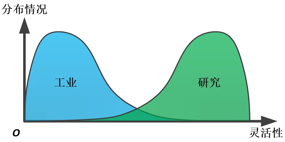
How industrial applications and academic research sit differently on the spectrum of robot flexibility.
What motion planning sets out to do is turn "motion-level programming" (teaching point after
point) into "task-level programming" (just say "grab A and put it at B," and the robot works out
the trajectory itself). If this technology were mature enough, users wouldn't need to know the
details of operating a robot — they'd just enter a task command; combined with visual
perception, it could even adapt to changes in the environment and the workpiece.
Let's state the problem clearly. Motion planning: given two points A and B in the robot's
configuration space, find a path between A and B that satisfies the constraints.
While we're here, let's clear up a naming confusion beginners often run into — what's the
difference between path planning, trajectory planning, and motion planning?
Path planning plans a spatial route \(\theta(s)\) (\(0 \le s \le 1\)), with no time
information; it addresses reachability;
Trajectory planning plans \(\theta(t)\), with timestamps; it addresses differential
constraints related to time, velocity, and so on;
Motion planning is the broader concept: its output can be discrete waypoints, a continuous
path, a time-stamped trajectory, or even a control policy.
The definitions themselves don't matter much; what matters is being clear about who does what in
the system. For the simplest task (get from A to B avoiding obstacles), the planner outputs a
geometric path and the robot's controller handles the trajectory interpolation and closed-loop
control on its own — that's enough; for tasks with trajectory requirements (a fixed cycle time,
constant end-effector speed), path planning and trajectory planning have to work together; and
if the trajectory itself must satisfy dynamic constraints, the planner often has to compute the
trajectory directly, rather than splitting it into two steps.
To judge a planning algorithm, you usually look at two metrics — and for each new algorithm you
meet from here on, I'd suggest asking these two questions first:
Completeness: as long as the problem has a solution, the algorithm is guaranteed to find
one in finite time;
Optimality: the path found is optimal under a given metric (shortest, most
energy-efficient, etc.).
In the introductory part we discussed everything in the workspace, but the first step in motion
planning is to think in a different space.
The vector of a robot's joint angles is called the robot's generalized coordinates; the
space those generalized coordinates live in is the robot's configuration space (C-Space). In
C-Space, no matter what the robot looks like, it's just a single point — and that's exactly
the premise that lets various general planning algorithms be reused (A*, RRT, and the like are
all designed for point-like agents).
Planar mobile robot: inflate the obstacles by the robot's size (a Minkowski sum), and the
robot becomes a point on the \((x, y)\) plane; its C-Space looks a lot like the workspace;
Serial arm: the C-Space is the joint space. Note that its topology is completely different from
the workspace — because a revolute joint's \(0 = 2\pi\) wraps around end to end, the C-Space of a
two-DOF arm is actually a torus; the C-Space of a general serial arm is a manifold.
Why insist on planning in C-Space? Because the mapping from C-Space to the workspace (forward
kinematics) is surjective, so a planning result is always executable; the reverse (inverse
kinematics) has issues like multiple solutions and singularities, so a result planned in the
workspace might not be executable at all. So, for a robot arm, in principle all the work can be
done entirely in C-Space.
But the price is dimensionality. Add one rotational DOF to a mobile robot and A*'s search
difficulty multiplies; by the time you reach a six-DOF arm, discretizing the C-Space at a 6°
resolution produces \(60^6 \approx 4.7 \times 10^{10}\) cells — even if each collision check took
only 0.1 ms, one full sweep would take 1296 hours. Motion planning is NP-hard, its complexity
growing exponentially with dimension; this is the "curse of dimensionality," and it's the source
of every difficulty in this field.
Two footnotes. First, the notion of C-Space is the theoretical bedrock of this field; I've always
recommended Principles of Robot Motion[8] for getting started — for no other reason
than that it puts C-Space in a suitably important place, rather than launching straight into RRT.
Second, the C-Spaces of common mechanisms are all Lie groups — a multi-joint robot is a Torus(n),
a drone is SE(3) — and the last chapter's unified sampling and interpolation definitions let the
same planning algorithms run on all of these spaces (which is precisely how the State Space is
designed in OMPL).
The map of algorithms: sampling, optimization, learning
There are countless planning algorithms, but from a methodological angle they fall into roughly
three big classes. I'll give you the map, not the details — the principle of each algorithm is
laid out clearly in the textbooks[8][9] and the OMPL
docs; years ago I also wrote a more detailed piece,
Motion Planning: An Introduction (in
Chinese), going from pathfinding in Red Alert to robot arms.
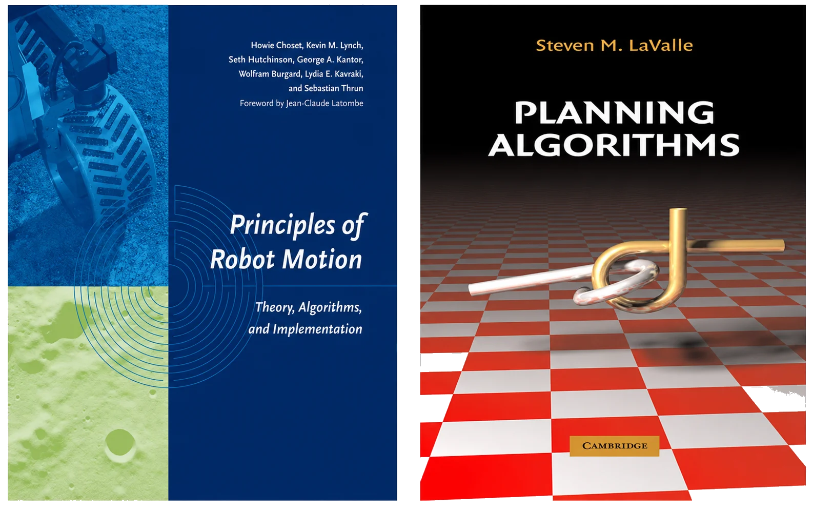
Some motion-planning textbooks.
Graph-search-based methods (strictly speaking, the shared foundation of all three classes):
turn the C-Space into a graph of nodes and edges, then use Dijkstra or A* to find the shortest
path. Ways to build the graph include the visibility graph (complete and optimal in 2D), grid
discretization (resolution complete — too coarse a grid can wall off a passage that actually
exists), and so on. They work very well in low-dimensional spaces — pathfinding in real-time
strategy games and mobile-robot navigation are basically this routine — but, limited by the curse
of dimensionality, they don't scale to a six-DOF arm.

Dijkstra vs. A* search, side by side.
Optimization-based methods: treat the trajectory as the variable, write an objective function,
and optimize it directly. The forefather is Khatib's artificial potential field — its cleverness
is that it doesn't care about C-Space topology at all, computing virtual forces in the workspace
and converting them into joint torques, which makes it fast enough to go inside a real-time
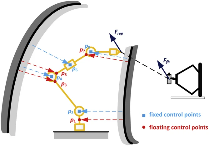
control loop; for a high-DOF arm, you can place several control points along the arm and apply
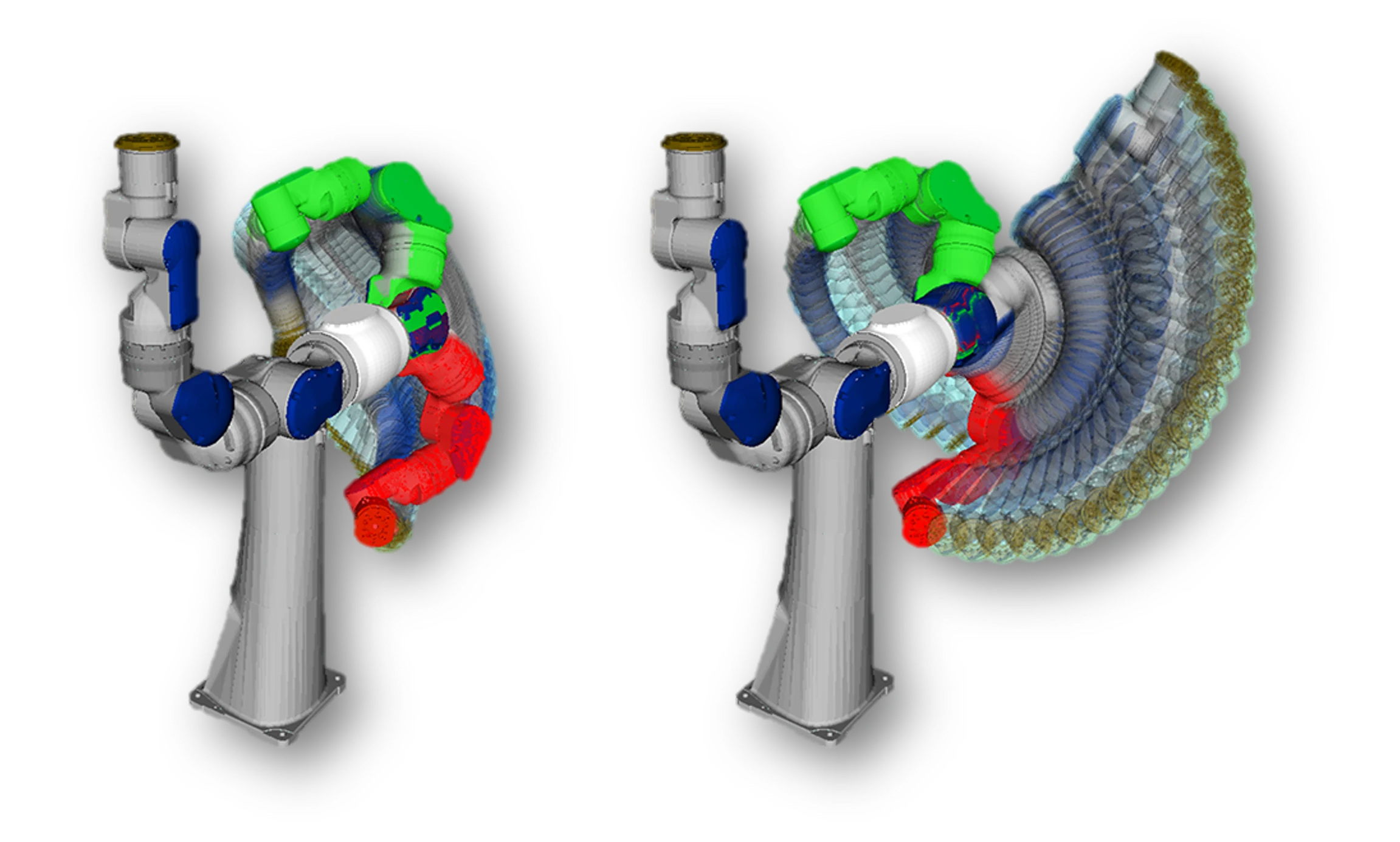
forces to each (the figure below is from my own paper). The later CHOMP (precomputed
obstacle-distance field + gradient descent), STOMP (random perturbations, gradient-free), and
TrajOpt (SQP + continuous collision detection via convex decomposition) all belong to this
category. Their shared problem is local minima: the planning problem is inherently non-convex,
and optimization can only give you "the best answer nearby."
Control-point-based artificial potential field: workspace virtual forces are converted into joint torques through the Jacobian.
Sampling-based methods: since C-Space is hard to describe explicitly, don't describe it — just
run collision checks on random sample points. PRM first scatters random points to build a graph,
then queries it; RRT grows a random tree from the start point, skipping the learning phase and
adapting better to dynamic environments; the follow-ups — RRT-Connect (bidirectional growth,
still one of the most efficient solvers to this day), RRT*/PRM* (asymptotically optimal), and
the Lazy family (deferred collision checking) — are all improvements on these two frameworks.
This class of methods is probabilistically complete, not optimal, plans fast, and is
currently the mainstream choice for arms with six or more DOF.


An arm avoiding obstacles, planned by a sampling-based algorithm.
Learning-based methods: a more precise name would be "data-driven methods" — the essence is
"distilling" experience, rules, and evaluation criteria from data so as to react quickly in new
scenarios. From the earliest learning from demonstration (LfD/DMP, fitting human-taught
trajectories with a Gaussian mixture model) and imitation learning, to today's red-hot
reinforcement learning, VLA, and other "embodied AI" techniques — all belong to this category. As
research has advanced, this has become the field of the moment, and a hotly contested one. We'll
save the specifics for later.
The planner gives a geometric path; what the robot actually executes is a time-stamped trajectory.
Trajectory planning can be split into two parts — path interpolation and time computation:
first obtain the geometric path \(p(u)\), then decide the speed at which to traverse it, i.e.
\(u(t)\). For this part I recommend a dedicated textbook: Biagiotti and Melchiorri's Trajectory
Planning for Automatic Machines and Robots[10].
Joint-space interpolation (trapezoidal velocity profiles, splines) you've already seen in the
introductory part; Cartesian-space orientation interpolation, on the other hand, has a pitfall —
Slerp guarantees only first-order continuity, and higher-order-continuous blends need Lie-group
tools, which the last chapter's "orientation interpolation and trajectory blending" already
covered, so I won't repeat it.
There's a fact on the time-computation side worth thinking hard about: when we do trajectory
planning for a robot controller, we're used to giving velocity and acceleration constraints — but
there's actually no such thing as a velocity or acceleration constraint in a robot system. Every
operation we perform acts on motor torque; all we have is a torque constraint. So, under a
torque constraint, how do you make the robot traverse a given path as fast as possible? That's
time-optimal trajectory planning (keyword: time-optimal path parameterization), and it's another
place where numerical optimization shines.
One more thing from engineering: the path a sampling planner computes is often redundant and full
of kinks, and executing it directly looks ugly. The standard approach is a three-step
post-processing — path shortcutting (removing unnecessary detours), trajectory optimization
(optimization-based algorithms), and trajectory planning (time parameterization) — converting it
into a trajectory the controller can execute.
But there are actually plenty of details left: do the later processing steps change the shape of
the trajectory, and if so, how do you keep it collision-free? When there are many points, sticking
as strictly as possible to the planned path may mean you can't hit the optimal cycle time; to push
the cycle time further, you have to adjust the trajectory shape more aggressively.
So, going a step further, you can put the position and velocity of the whole trajectory into one
global optimization problem and tune them together: from the same geometric path, you can optimize
out trajectories that are optimal under different constraints — time-optimal, collision-free,
constant end-effector speed, and so on.
Now let's look at a real industrial task. Arc welding requires the torch tip to move along the
weld seam with its axis held in a specified direction — but rotation about that axis is free;
assembly and grinding are similar; the last chapter's high-speed transport constrains acceleration
and orientation, but places no requirement on position. In other words: most tasks don't pin
down all of the robot's degrees of freedom; the system is under-constrained. These extra degrees
of freedom are the room the planner has to move in.
The most direct tool is the null space. When the task needs only \(m\) degrees of freedom and
the robot has \(n\) (\(m < n\)), the velocity-level inverse kinematics \(J\dot{q} = \dot{x}\) is
underdetermined, and the general solution is:
\[\dot{q} = J^{\dagger}\dot{x} + (I - J^{\dagger}J)\,v\]
The second term is null-space motion: the robot moves, yet the end-effector doesn't budge an inch.
Note that "redundant" doesn't specifically mean seven axes — a six-axis arm doing arc welding (a
task that constrains only five DOF) is a redundant robot too. A seven-axis arm just takes this to
the configuration level: the same end-effector pose corresponds to infinitely many
continuously-distributed inverse solutions (self-motion), so you can hold the end-effector
trajectory while dodging singularities, joint limits, and obstacles — which is exactly why every
vendor has rolled out a seven-axis product. For more, see
Curious about seven-axis arms? (in Chinese).
A seven-axis arm uses null-space self-motion to dodge an obstacle while keeping the end-effector pose fixed.
Project the gradient of an optimization objective (stay farther from joint limits, farther from
obstacles, higher manipulability) into the null space, and you get the classic gradient-projection
method — simple enough to embed in a real-time control loop. But it's essentially local gradient
descent, so it gets stuck in local minima. To do global constrained planning, there are roughly
three routes:
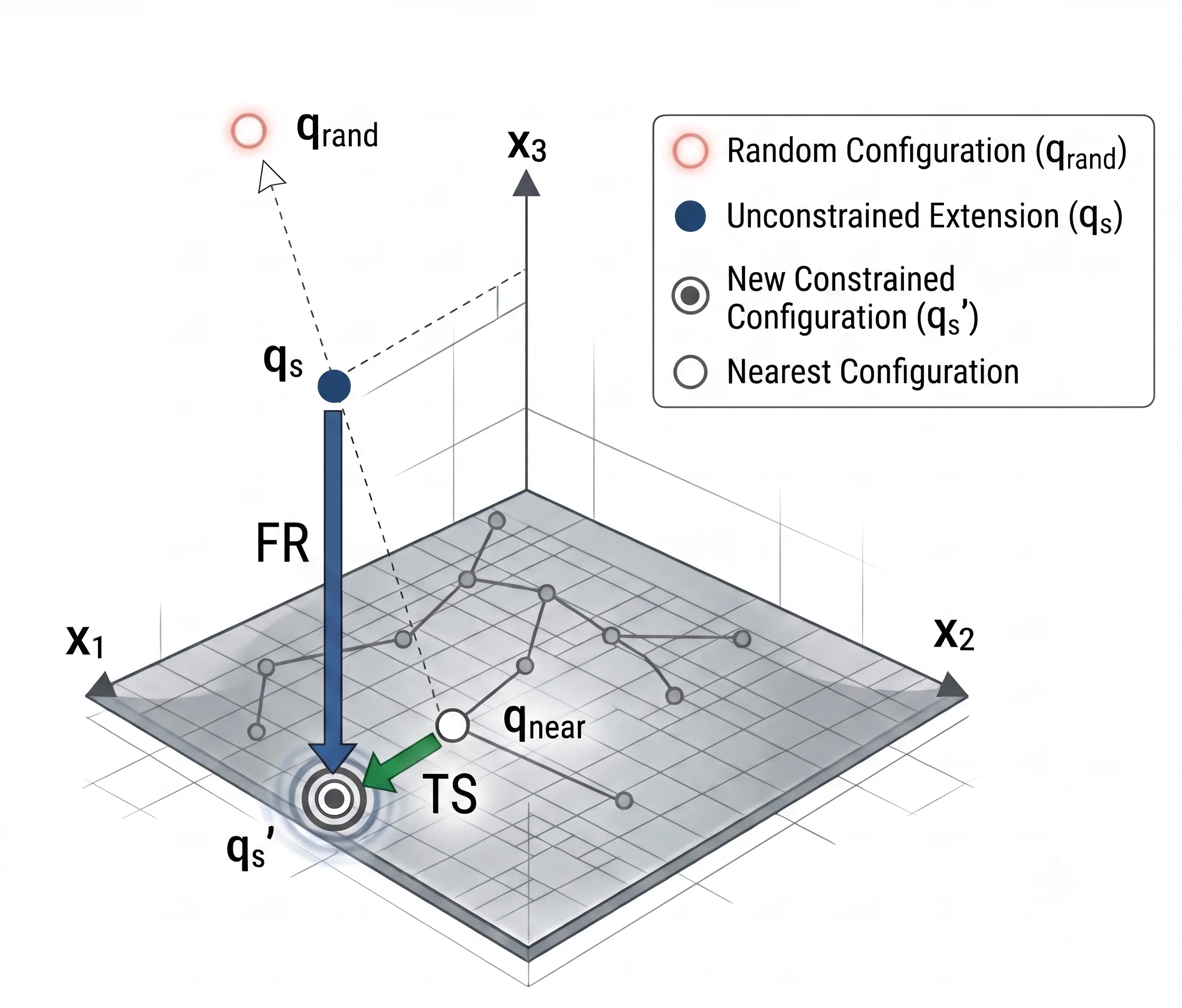
Sample + project: sample randomly in C-Space, project the samples onto the constraint-
satisfying manifold, then connect adjacent states with Jacobian iteration (the work of Stilman,
Berenson, and others; implemented in OpenRAVE);
Sample-and-project RRT planning under a task constraint.
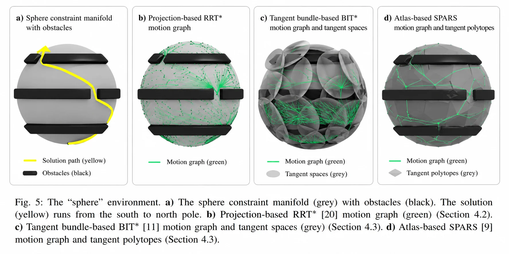
2. Grow directly on the manifold: e.g. Tangent Bundle RRT[11] and
AtlasRRT[12], building local coordinate charts for the constraint manifold as you
plan;
AtlasRRT: building an atlas on the constraint manifold while planning.
3. Explicit dimension reduction: look at it another way — an equality constraint reduces the
dimension of the space, so if you can explicitly construct the "low-dimensional space that
always satisfies the constraint," then anything you do inside it is legal, and the problem
actually gets simpler — you can even invite back old friends like A* and RRT. The last
chapter's high-speed transport did exactly this: a six-DOF problem with dynamic constraints
was reduced to a three-DOF problem in \(R(3) \oplus SO(3)\).
So far it's all been algorithms. But if you've been to a factory, you'll notice an awkward truth:
almost no robots on real production lines use real-time motion planning. At the Amazon Picking
Challenge (APC), faced with the narrow opening of a shelf, mainstream planners either couldn't
find a solution or were too slow to use, and the top-ranked teams almost all fell back to
"predefined keypoints + Cartesian interpolation"; plenty of commercial "smart" sorting systems
have no motion-planning module at all. It took MUJIN five years to build academic planning
technology into an industrial controller.
Where's the problem? Beyond the curse of dimensionality, there's randomness: algorithms like
RRT give a different solution for the same problem every time, and the planned motion often comes
with unnecessary wiggling — while industry is obsessed with stability and predictability.
A sampling planner solving the same task several times gives completely different results.
My entry point during my PhD was noticing that industrial environments are semi-structured:
most of the scene around the robot is fixed, and only the pick and place positions vary within a
small range. Given that, planning from scratch every single time is unwise — a past successful
trajectory very likely lies in an obstacle-free, and fairly good, region. Fit the historical
trajectories with a Gaussian mixture model (GMM) to get the feasible region in C-Space, then use
it to guide the random planner's sampling — that's the "experience roadmap" method. A number to
put on it: for an automotive spot-welding task, spend 48 hours offline computing 10 fairly good
trajectories with RRT* as experience; afterward, planning a full trajectory through 10 weld
points takes three minutes on average, at a 90% success rate — on the same problem, RRT-Connect
has only a 60% success rate and takes more than four times as long. Prior knowledge + a random
planner is the key step to getting planning technology onto the production line.
Another direction is to make "planning" a policy: when the environment is moving, you can't
wait for a full trajectory to finish computing before you move — you return, in real time, an
action that satisfies the constraints given the current state, i.e. a motion policy. Model each
task objective (reach toward the target, avoid obstacles, avoid joint limits, comply with
external forces) as a dynamical system on a different manifold, then combine them by
state-dependent priorities, and the robot can track its target while "gracefully" dodging
obstacles. For this, see Tech talk: real-time motion planning
(in Chinese).
Real-time motion planning: the arm tracks a target pose while dodging obstacles and singularities.
Of course, today's VLA and similar techniques are, at bottom, a kind of "motion policy" too — only
learned, and hoping to combine vision and language to learn a more general, more transferable
policy.
By the way: follow this "solve in real time every cycle" idea into the control field and you arrive
at Model Predictive Control (MPC) — each control cycle, solve a short constrained trajectory
optimization online, execute only the first step, and roll forward again next cycle (receding
horizon). See — the boundary between planning and control has already blurred here. Honestly, my
own hands-on experience with MPC is limited, so I won't pretend to be an authority; if you want to
go deeper, see Borrelli et al.'s textbook
Predictive Control for Linear and Hybrid Systems;
and its head-to-head comparison with reinforcement learning for whole-body control of humanoid and
legged robots, I'll leave for the Embodied AI part.
A one-liner on tools: if you want to get going fast, just use MoveIt (you can get planning running
in simulation in half an hour).
Finally, let's look at planning through a different lens. Motion planning is a textbook Markov
decision process (MDP): the state is the configuration, the action is the motion, and the reward is
"reach the goal without collision." If you deeply understand the algorithms that solve
reinforcement learning, you'll find that dynamic programming's (DP) iterative process works in
essentially the same way as Dijkstra — one computes from the goal backward, the other from the start forward;
and RRT* can be seen as one realization of the Monte Carlo idea. Reinforcement learning just
stores the policy and value in a "table," as its understanding of the environment, to speed up
planning.
Naturally, someone thinks: fit that table with a deep network, have the network output actions
directly, and planning time becomes a single forward pass — that's the motivation for doing planning
with deep reinforcement learning. I've tried it myself on bin picking: for visual-servoing-style
tasks it worked surprisingly well, but think about it carefully and that impressive-looking DRL was
really just fitting a Jacobian matrix; whereas for tasks that genuinely need to weave around obstacles in C-Space, all
it had left was "the trend is right, occasionally correct." So when judging this kind of work, it's
worth applying one criterion: how would a traditional method do this? If a traditional method
could do it in two lines of formula, then the learning hasn't created any added value yet.
Of course, that's just a glimpse from the planning angle. Data-driven methods have stirred up a far
bigger wave in robotics in recent years — their potential and their pitfalls, I'll save for the
Embodied AI part.